Graph theory primer
By Maria Sevillano
September 19, 2021
Aim
In this blogpost, I will review foundational concepts underlying co-occurrence networks and apply them to visualize a drinking water metagenome dataset.
Scope
The information discussed in the “Background” section is in part a summary of the “Graph Theory for Data Science” workshop series taught by Stanford University PhD student Julia Olivieri, as a part of Women in data science workshop series. Her workshops are available on youtube and consist of the three parts:
Part III: Characterizing Graphs in the Real World
In May 2019, I was one of the workshop organizers for Meta-omics in Environmental Engineering Research at the Association of Environmental Engineering and Science Professors (AEESP) conference. The slides I presented there are shared within this post as well.
Additionally, the plugging CoNet in the Cytoscape application will be used to infer associations between metagenome assembled genomes (MAGs) from drinking water systems.
The main objective of this post is to use R packages to describe and visualize the network.
Background
Graphs are structures that represent relationships between things.
The formal definition of a graph, G is
\[ G = (v,E) \]
the set of vertices, v (i.e., nodes), and edges, E (i.e., links) such that v is finite and non-empty and each element of E is a two-element subset of v.
In order to describe the topology of the graph we rely on different scores. Centrality measures, for example, are useful to determine the importance of nodes and edges compared to the remaining components of the graph.
Definitions
At the most basic level, the degree of a vertex gives an indication of how “central” it is, and how it connects to others. We just count the connections to a node and voila. This is a local measure that is easy to calculate and high degree nodes are considered “hubs”. However, the inability to uniquely rank nodes is very likely.
Alternatively, global connectivity measures consider the node’s neighbors. One such measure is eigencentrality (i.e., eigenvector centrality). This score accounts for the degree of the node as well as the degree of connected nodes (i.e., neighbors). The relative centrality score of vertex v with neighbor t can be defined as:
\[ x_v = \frac{1}{\lambda}\sum_{t{\in}M(v)}x_t \]
where M(v) is a set of the neighbors of v and is a constant.
Other global scores that are more widely used are closeness centrality and betweenness centrality, both of which rely on path length information. Closeness centrality is a measure of how close a vertex is to the other vertices by summing the shortest path distances. Formally,
\[ \frac{N-1}{\sum_{j} d(i,j)} \]
where N is the number of nodes. It is the reciprocal of the average shortest path length.
Alternatively, betweenness centrality scores place emphasis on the shortest path a node is part of. Higher scores correspond to nodes that are gatekeepers of information flow. It is defined as follows:
\[ \sum_{j<k} \frac{g_{jk}(n_i)} {g_{jk}} \]
Vocabulary
- walk: sequence of vertices connected by edges.
- trail: walk with no repeated edges.
- cycle: non-empty trail that starts and ends at the same vertex.
- connected: if a vertex can be reached from any other vertex through a walk.
- tree: a connected graph that doesn’t contain any cycles.
- degree: number of edges connected to vertex.
- sub-graph: subset of vertices and corresponding edges.
- complete graph: contains an edge between every pair of vertices (degree of each vertex in n-1, where n is the number of vertices).
- clique: the largest complete sub-graph.
- adjacency matrix: matrix with rows and columns labeled by graph vertices, with a 1 or 0 in position (v_i,v_j) according to whether v_i and v_j are adjacent or not.
There are multiple types of graphs that we might be familiarized with. For example, phylogenetic trees show ancestral relationships between taxa, chemical structures show connection between molecules, and co-occurrence networks are representations of the relationships between biological entities within a context. In this post, I will be describing the co-ocurrence network of metagenomes from drinking water systems.
There are a few tools at our disposal for co-occurrence inference from sequencing data, but I’m more familiar with CoNet. This tool detects non-random patterns of co-occurrence in presence/absence and abundance data based on user selected thresholds.
The general workflow is:
Preprocessing
raw data matrix is processed by removing rare taxa, and normalizing counts
Edge score computation
pairwise scoring using a range of measures (i.e., ensemble method) to capture different types of relationships
Significance assessment
Computation of p-value using a Z-test, comparing the permutation distribution mean given the bootstrap distribution
CoNet runs on command line and as a Cytoscape plugin, there is also an R implementation, but is not on CRAN or continuously maintained.
Libraries
library(tidyverse)
library(visNetwork)
library(igraph)
Data wrangling
The tables resulting from the CoNet workflow require minimal wrangling. Here’s a sneak peak of the node and edge tables, respectively.
## # A tibble: 6 x 2
##   id      value
##   <chr>   <dbl>
## 1 DW01178    22
## 2 DW01233    20
## 3 DW01231    20
## 4 DW01139    20
## 5 DW01202    19
## 6 DW01177    18
## # A tibble: 6 x 5
## from to weight interactionType color
## <chr> <chr> <dbl> <chr> <chr>
## 1 DW01142 DW01102 0 copresence #00b300
## 2 DW01132 DW01177 0 copresence #00b300
## 3 DW01235 DW01225 0 copresence #00b300
## 4 DW01178 DW01202 0 copresence #00b300
## 5 DW01233 DW01138 0 copresence #00b300
## 6 DW00423 DW00424 0 copresence #00b300Analyses
A high level summary of network metrics are shown below:
| Network properties | |
|---|---|
| Global information | |
| property | value |
| Clustering coefficient | 0.329 |
| Connected components | 30.000 |
| Network diameter | 15.000 |
| Network radius | 1.000 |
| Network centralization | 0.076 |
| Characteristic path length | 5.012 |
| Number of nodes | 232.000 |
| Average degree | 4.517 |
| Network density | 0.020 |
For a comprehensive description of metrics and their interpretation, take a look a this site.
Let’s see what the network looks like!
In this network, positive and negative type interactions are colored green and red, respectively.
I’ve also created this shiny app to play with the network’s layout. Take a look!
From the network graph we can see that there are two large components (or clusters), in fact 71.12% of the MAGs are part of those clusters.
We will now hone in on these nodes by creating two connected sub-graphs.
As discussed in the ?? section, we can use centrality measures to describe node importance.
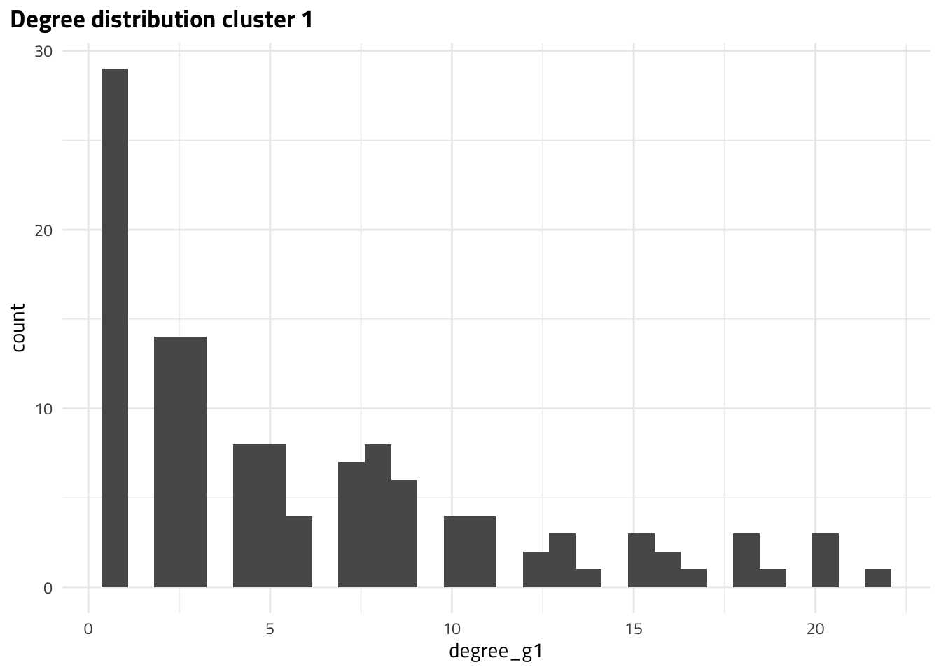
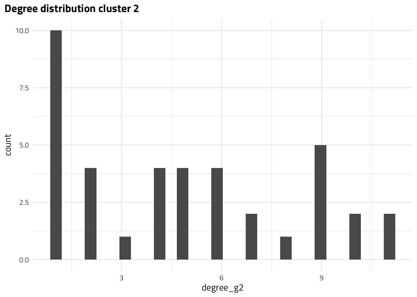
The MAGs with largest degrees correspond to DW01178 and DW00270, DW00626 in cluster 1 and 2, respectively. However, we know that degree alone is not the best metric for node importance. Let’s take a look at global metrics of centrality.
The highest ranking MAGs for each metric in terms of centrality are
| Centrality metric ranking | |
|---|---|
| node | value |
| Cluster 1 - betweenness | |
| DW00520 | 3611.2821 |
| DW01139 | 2585.2435 |
| DW01220 | 2459.7131 |
| DW01169 | 1803.8373 |
| DW01102 | 1746.3667 |
| Cluster 2 - betweenness | |
| DW00270 | 257.6060 |
| DW00428 | 161.8021 |
| DW00626 | 122.4988 |
| DW00462 | 106.8060 |
| DW00424 | 103.1034 |
| Cluster 1 - degree | |
| DW01178 | 22.0000 |
| DW01233 | 20.0000 |
| DW01231 | 20.0000 |
| DW01139 | 20.0000 |
| DW01202 | 19.0000 |
| Cluster 2 - degree | |
| DW00270 | 11.0000 |
| DW00626 | 11.0000 |
| DW00426 | 10.0000 |
| DW00424 | 10.0000 |
| DW00462 | 9.0000 |
| DW00440 | 9.0000 |
| DW00428 | 9.0000 |
| DW00988 | 9.0000 |
| DW00427 | 9.0000 |
| Cluster 1 - eigenvector | |
| DW01178 | 1.0000 |
| DW01139 | 0.9191 |
| DW01231 | 0.9139 |
| DW01202 | 0.9120 |
| DW01155 | 0.8747 |
| Cluster 2 - eigenvector | |
| DW00424 | 1.0000 |
| DW00428 | 0.9595 |
| DW00440 | 0.9517 |
| DW00988 | 0.9486 |
| DW00462 | 0.9091 |
| Cluster 2 - closeness | |
| DW00428 | 0.0132 |
| DW00462 | 0.0127 |
| DW00270 | 0.0127 |
| DW00479 | 0.0125 |
| DW00626 | 0.0122 |
| Cluster 1 - closeness | |
| DW01139 | 0.0024 |
| DW01178 | 0.0023 |
| DW01233 | 0.0023 |
| DW01155 | 0.0023 |
| DW01231 | 0.0023 |
| DW01138 | 0.0023 |
| DW01145 | 0.0023 |
Further, higher level metrics for both subgraphs are provided below.
| Network properties of subgraphs | ||
|---|---|---|
| Global information | ||
| property | Cluster 1 | Cluster 2 |
| Clustering coefficient | 0.406 | 0.358 |
| Network diameter | 15.000 | 7.000 |
| Network radius | 8.000 | 4.000 |
| Network centralization | 0.127 | 0.161 |
| Characteristic path length | 5.226 | 3.007 |
| Number of nodes | 126.000 | 39.000 |
| Average degree | 6.127 | 4.872 |
| Network density | 0.049 | 0.128 |
- Posted on:
- September 19, 2021
- Length:
- 16 minute read, 3197 words
- See Also: